Ordinary Differential Equations

An ordinary differential equation is a differential equation in which all dependent variables are functions of a single independent variable. ODEs show up all over the place in physics. From analyzing Newton’s laws, to harmonic motion, to circuit analysis, these types of problems are very common and are typically encountered with when working on realistic physical systems.

For a given ODE, if it is reduced to its simplest form, the highest derivative (first, second, etc.) tells us the “order” of the ODE. In general, we would like to be able to describe an algorithm that enables us to solve an \(n^{th}\) order ODE. As an example, consider

\[\frac{d^2x_j}{dt^2}=\frac{F_j(x_1,...,x_n,t)}{m_j}\]

where \(x_j\) is the position of the \(j^{th}\) object, \(m_j\) its mass, and \(F_j\) is the net force acting on that object, which may depend on any number of other variables (\(x_i, t, \) order ODE as a series of n 1:math:^{st} order ODEs and apply techniques that can solve just 1:math:^{st} order equations. For example, we can rewrite our equation above as

\[\begin{split}\frac{dx_j}{dt} &= v_j,\\ \frac{dv_j}{dt} &= \frac{F_j(x_1,...,x_n,t)}{m_j}\end{split}\]

As a shorthand, let’s denote our first derivative using prime notation: \(y'\). We are given the ODE as a function of some number of independent variables:

\[y'=\frac{dy}{dx}=f(x,y,...)\]

where in this case, we let the prime denote that we are taking the derivative with respect to x. Again, we know \(f(x,y,...)\) and we seek the solution to the ODE: \(y(x,...)\). In other words, we know the derivative of y, which is a function of y and other variables, we want to find y as a function of those other variables.

Note

For all of the methods discussed here, I’ve tried to assume that our ODEs are a function of a general number of variables. Of course, it is possible that any given ODE only be a function 1 (or even no) variables.

For any technique, in order to solve this equation, we need some other information about our function \(y(x,...)\). Typically, we are given some initial value boundary condition. For example, let’s assume that the function that we are after is only a function of a single variable, such that \(y = y(x)\). Then, we may be given

(1)\[y(x_0) = y_0\]

the value of the function \(y\) at some location. In order to find the value of \(y\) at all other locations, we must use this value. As is the case for many of the problems that we deal with in this course, before we can proceed, we need to discritize the domain that we are interested in. In other words, we will find \(y\) at all points \(x_i\) where

\[x_i = x_0+ih\]

and \(h\), as always, is the grid spacing. Given the ODE, an initial value and a grid, we can then proceed to implement a few different techniques to solve our ODE.

Euler’s method

The most basic technique that we can employ to solve our \(1_{st}\) order ODE is Euler’s method. This technique exploits the fact that we know the 1st derivative of a function, \(y'(x)\) and an initial value of the function itself, \(y(x_0)\). We then find the value of the function at a neighboring point, \(y(x_1)\) by assuming that the derivative is constant between the two grid points \(x_0\) and \(x_1\). We can write the technique as:

(2)\[y_{n+1} = y_n+y_n' h\]

Since we are given information about \(y'\) everywhere, we can determine \(y_{n+1}\) if we know \(y_n\). Thus we require the boundary condition in Eq. (1). This process is depicted graphically below.

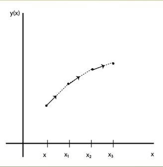
We are given \(y(x_0)\) and from there we can use information about the derivative of y to find subsequent values of y.

In Eq (2), it may seem as though we don’t use information about the grid. However, remember 1) that we must know \(y_0\) at some initial value for \(x\) at \(x_0\) and 2) our ODE, \(y'(x,...)\) may also be a function of \(x\). Generally, Euler’s method is relatively straightforward to implement.

1. Establish a grid that spans the domain of interest.
2. Initialize variables, including specifying the initial value condition according to Eq (1).
3. Create a loop that covers each grid point.
4. Evaluate the value of the ODE, \(y_i'\) at that grid point, \(x_i\) given \(y_i\) .
5. Apply Eq (2) to find the value of the function, \(y_{i+1}\) at the next point.
6. Repeat until you’ve reached the end of the grid.

Although the algorithm is relatively simple, there are 2 issues to consider: 1) error and 2) stability.

Runge-Kutta Techniques

The methods that are typically used by scientists to solve ODEs are called Runge-Kutta schemes (after a couple German mathematicians). The idea is this: since Euler’s method is asymmetric, it only depends on derivatives taken at the beginning of a particular interval of interest. This makes the errors relatively high. Runge-Kutta methods attempt to perform a more symmetric step. First, take an Euler step to the midpoint of the interval:

\[y_{n+\frac{1}{2}} = y_n+y'\frac{h}{2}\]

Then, use the values at that point to calculate the solution at the real interval. This results in the \(2^{nd}\) order Runge-Kutta method. Given some ODE that is a function of some number of variables, \(y'(x,y,...)\):

\[\begin{split}k_1 &= hy'(x_n,y_n,...)\\ k_2 &= hy'(x_n+h/2,y_n+k_1/2,...)\\ y_{n+1} &= y_n+k_2+\mathcal{O}(h^{3})\end{split}\]

The result of this is the first order errors are canceled out and we get a method that is \(2^{nd}\) order accurate. We gain accuracy by using the derivative evaluated at an extra point, and by being smart about it.

Of course, we don’t need to stop at taking the derivative at just one extra point. We could keep going! In fact, the \(4_{th}\) order Runge-Kutta method is one of the most popular methods of integrating ODEs currently in use:

(3)\[\begin{split}k_1 &= hy'(x_n,y_n,...)\\ k_2 &= hy'(x_n+h/2,y_n+k_1/2,...)\\ k_3 &= hy'(x_n+h/2,y_n+k_2/2,...)\\ k_4 &= hy'(x_n+h,y_n+k_3,...)\\ y_{n+1} &= y_n+\frac{k_1}{6}+\frac{k_2}{3}+\frac{k_3}{3}+\frac{k_4}{6}+\mathcal{O}(h^5)\end{split}\]

The \(4^{th}\) order RK method isn’t necessarily limited by round off error as you increase \(n\), but rather, the computational effort. For every step, the ODE must be evaluated 4 times (or in general, \(n\) times for an \(n^{th}\) order RK method). As \(n\) gets large, this means many calculations are performed for each step. For this reason, higher order methods are not frequently used. They don’t give enough benefit in error reduction to make the decrease in performance worthwhile.

Implementation of Runge-Kutta techniques are very similar to that of Euler’s method. The difference being that we must evaluate the \(k\) values before we can find \(y_{n+1}\):

1. Establish a grid that spans the domain of interest.
2. Initialize variables, including specifying the initial value condition according to Eq (1).
3. Create a loop that covers each grid point.
4. Find \(k_1\) by evaluating the value of the ODE, \(y_i'\) at that grid point, \(x_i\) given \(y_i\).
5. Using the previous step, find \(k_{n+1}\) by evaluating the ODE using updated values. Repeat as necessary for remaining \(k\) s.
6. Apply final equation in Eq (3) to find the value of the function, \(y_{i+1}\) at the next point.
7. Repeat until you’ve reached the end of the grid.