Numerical Integration

In upper level physics, we constantly run in to integral problems that are difficult, if not impossible, to solve analytically. Systems that are more complex than the most basic examples often require the use of approximations that may not be applicable to a particular problem. Luckily, there exist a wide swath of numerical techniques that can be implemented to attack such problems. Here, we will cover a few of them as a study on how such techniques are developed and how to implement them. It should be noted that today’s computing languages often come with all, and more, of these techniques implemented in pre-existing software libraries.

Given some function \(f(x)\), we would like to find the solution the integral:

\[I = \int_a^bf(x) dx\]

Techniques for solving this problem all stem from the fundamental definition of the integral. Given some function, \(f(x)\), the integral is equal to the area under the curve defined by \(f(x)\) between the points \(a\) and \(b\). Our job is to use the computer to find a estimate for that area.

Numerically, this means that we have to break up the area into discrete chunks and sum the area of each chunk. The question is: how to break up each chunk?

Rectangular rule

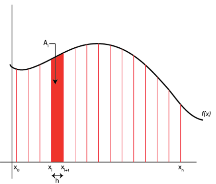
Since finding the area of a rectangle is pretty easy, perhaps the simplest method that we can choose would be to break up the domain that we are interested in into several rectangular chunks. This means that for each rectangle we must define the width of the rectangle (the difference between two points on our grid) and the height of our rectangle (the function evaluated at some point, \(f(x_i)\)). There are a few options when it comes to selecting the height.

Let’s say that I want to evaluate the area of the \(i^{th}\) rectangle. The width of my rectangle is \(x_{i+1} - x_i\). The height can either be defined using \(f(x_i)\) or \(f(x_{i+1})\). As you can see in the figure below, this will result in some error, either an underestimate of the true area or an overestimate depending on the behavior of the function.

Choosing the left point results in an overestimate.

Choosing the right point results in an underestimate.

This method of approximating the area under the curve is known as the rectangular rule. Once we set up a grid (\(x_0, x_1, x_2, \dots x_n\)) and evaluate our function at each point on the grid, it is easy to calculate the area of each rectangle and sum to get the integral. E.g. we can approximate the integral using the points on the left side of our rectangle using:

\[I=\sum_{i=0}^{n-1}f(x_i)h\]

A common adaptation to the rectangle rule is to use the midpoints of our grid as the point at which to evaluate the “height” of our function. If we don’t actually know the value of our function at those points, we can interpolate. This gives us the midpoint rule:

\[I = \sum_{i=0}^{n-1}f(\frac{x_i+x_{i+1}}{2})h\]

Trapezoid rule

It is clear from the above figures that there can be significant error when implementing the rectangular rule. An alternative then, is instead of breaking the domain up into rectangles, use trapezoids!

Trapezoids allow us to use information about the function at both grid points

Calculating the area of a trapezoid is not much more difficult that doing so for a rectangle, and the sum is similar:

\[I = \sum_{i=0}^{n-1}\frac{f(x_i)+f(x_{i+1})}{2}h\]

As you can see from this sum, the function is evaluated twice at each point on our grid, with the exception of the first and last

grid points. Written out, the sum looks like:

\[I = \left(\frac{f(x_0}{2}+f(x_1)+f(x_2)+\dots+\frac{f(x_n)}{2}\right)h\]

In this form, the trapezoid rule looks quite similar to the rectangle rule (and also the midpoint rule). The only difference being that we divide the function evaluated at the first grid point by 2, and add and extra term: \(\frac{f(x_n)}{2}\). This should tell you that while we might think the trapezoid rule is much more accurate that the rectangle rule, it actually isn’t that much better.

In fact, we can calculate the error of these two methods:

\[\begin{split}error_{midpoint} &\approx -\frac{h^3}{24}f''\\ error_{trapezoid} &\approx \frac{h^3}{12}f''\end{split}\]

where both error terms depend on the 2nd derivative of the function and the negative sign means that the approximation underestimates the solution when the function is concave up. By taking a weighted average of the two methods, we can effectively cancel out these errors and come up with a new method!

Simpson’s Rule

The weighted average looks like:

\[I_s = \frac{2I_m+I_t}{3}\]

where \(I_m\) represents the integral calculated with midpoint rule and \(I_t\) represents using the trapezoid rule.

Based on that formula, we can combine the summations above to write down the Simpson rule:

\[\begin{split}I&=\frac{h}{3}\left(f(x_0)+2\sum_{i=1}^{n/2-1}f(x_{2i})+4\sum_{i=1}^{n/2} f(x_{2i-1})+f(x_n)\right)\\ I&=\frac{h}{3}\left(f(x_0)+4f(x_1)+2f(x_2)+4f(x_3)+2f(x_4)+\dots+4f(x_{n-1}) +f(x_n)\right)\end{split}\]

Note that n must be even. This technique results in an error proportional to \(h^5\), which is much better than our options above. Additionally, the error depends on the fourth derivative of the function in question, which means that it is exact for any polynomial of 3 degrees or less, a nice bonus.

Implementation of Simpson’s rule is only slightly more complex than the rules above, only because the coefficient changes depending on if we are dealing with a odd or even grid point. There is a slight computational expense associated with performing the extra floating point operation. However, the improved accuracy over the midpoint method makes Simpson’s rule a good choice for typical integration tasks.

Monte Carlo techniques

The techniques discussed above are all based on the concept of interpolating the function that needs to be integrated in some way. However, there are other techniques that we can think of that attack the problem in a different manner. One class of such techniques are Monte Carlo methods, named because they involve some measure of randomness.

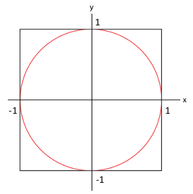
To illustrate the concept, imagine that you wanted to calculate the area of a circle, but you didn’t know anything about \(\pi\) or any of that. Instead, you chose to surround the circle by a square, for which you do know how to calculate the area. One might draw such a diagram on a piece of paper:

Next, we throw darts at the paper and we take a tally of total number of darts that were thrown as well as the darts that land inside the circle.

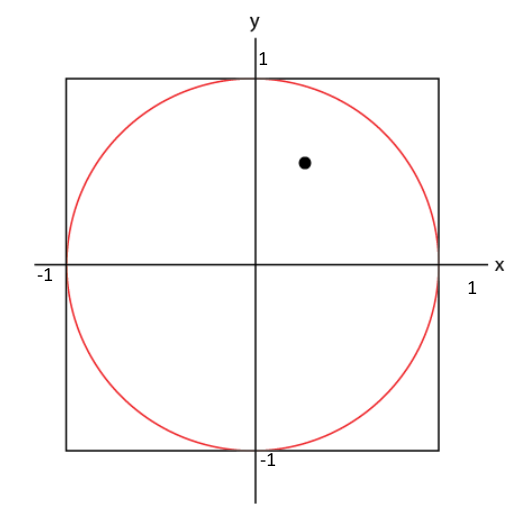
Inside the circle = 1, Total 1

Inside the circle = 2, Total 3

Inside the circle = 4, Total 7

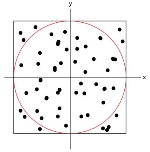
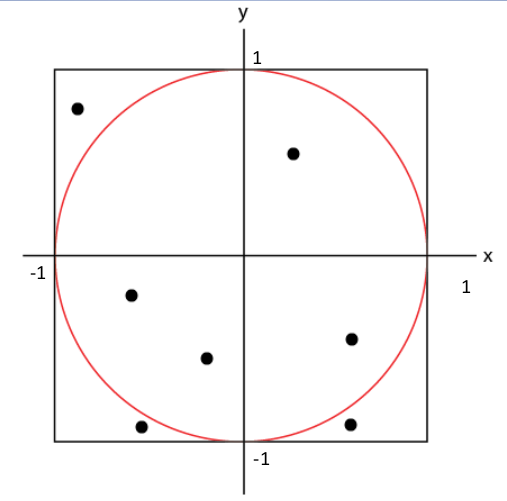
Inside the circle = 40, Total 50

So, 40 out of 50 darts are inside the circle, or 80%. So, assuming the darts were thrown randomly, I could approximate the area of the circle by \(a_c\approx 0.8A_s\).

If my square has an area of 4 units, then

\[A_c=4.0*0.8=3.2\approx\pi r^2=3.1415\]

Not a bad approximation!

In other words, I can implement this to find the integral of a function but picking a random coordinate \((x,y...)\) in the domain. Then, solve the function at that coordinate \(f(x)\). Assuming I am taking the integral with respect to \(y\), I could check to see if the random \(y\) value that I picked in the first step is less than f(x). If that is the case, I would tally that point as “in”. Repeat the procedure with some number, n, of random points. Then, the integral is approximated by the area (volume, etc) of the domain * in / n. Of course, the larger n, the better the approximation.

Monte Carlo techniques tend to be slower for low dimensional problems. If you are doing 1D or 2D integration, it is best to stick with Simpson’s rule if possible. However, if you have a higher dimensional problem, 3D, 4D, etc. then Monte Carlo methods can be extremely beneficial.